Conservation laws and Domain meshing for numerical simulations

Mass and momentum conservation

Any conservation law for fluid motion can be expressed in conservative formulation as a partial differential equation (PDE), that in case of a depth-averaged model (shallow water equations or SWE) in a 2D or X-Y plane is written as:

\[\frac{\delta \bar U} {\delta t} + \frac{\delta \bar F} {\delta x} + \frac{\delta \bar G} {\delta y}=\bar H\]

Where U is the vector of conservative variables, F and G are flows in X and Y directions respectively, and H is a source term. For the complete 2D Saint Venant equations the terms are:

\[ \begin{align}\begin{aligned}\bar U =(h, hU_x, hU_y)^T\\\bar F =(hU_x, hU^2_x+\frac{1}{2}gh^2, hU_xU_y)^T\\\bar G =(hU_y, hU_yU_x, hU^2_y+\frac{1}{2}gh^2)^T\\\bar H =(0, gh(So_x-Sf_x), gh(So_y-Sf_y))^T\end{aligned}\end{align} \]

Symbol	Variable and dimension	Symbol	Variable and dimension
h	water depth (m)
Ux	X-velocity (m/s)	Uy	Y-velocity (m/s)
Sox	X-Slope (no dim)	Soy	Y-Slope (no dim)
Sfx	X-friction slope (no dim)	Sfy	Y-friction slope (no dim)
g	gravity constant (m/s^2)

The differential solvers are evaluated across neighbouring cells of a domain or mesh, that historically have been evolving from quadrilateral to triangular shapes. As first example, the raster based approach used by Lisfloood-FP is presented:

Type of mesh

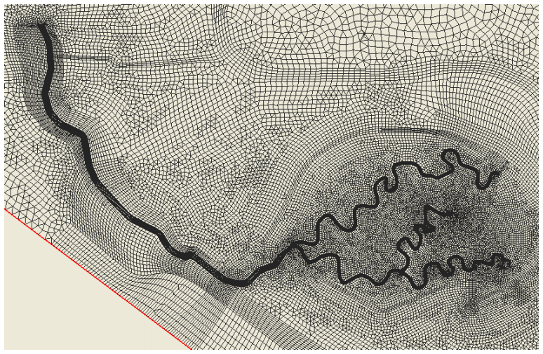
Triangular based meshes for 2D domains, to discretize the mass and momentum differential equations. As example, the non-structured triangle based approach used by RiverFlow2D, a Delaunay tessellation:

Practical approach: hybrids

The river main channel interaction with the floodplain by overtopping embankments or levees can be modelled using a combination of cells (quadrilateral or triangular) which will require higher density of cells in the transitions or when the speed pattern is expected to be more complex or less uniform in space. The whole domain can be seen as a 1D conduit plus a 2D plain:

Or as a complete 2D domain, which is easier to config and more stable, but demands more memory and CPU time. For instance RSH-2D (US Bureau of Reclamation, 2008) combines quadrilateral cells along the main channel and levees but mixed coarser cells at the plains.

Or the widespread non-structured triangular mesh for the whole domain, also known as flexible mesh, note the finest resolution around levees, by TELEMAC model.

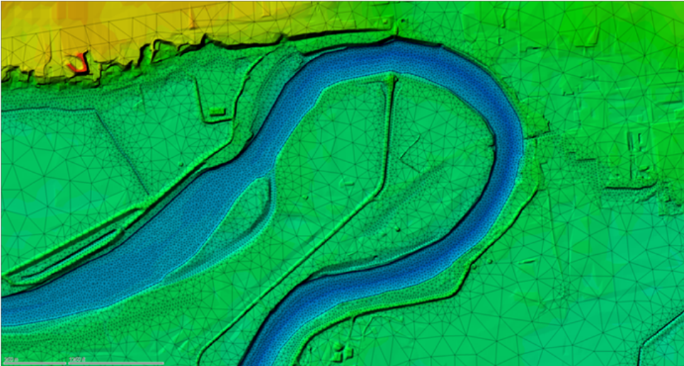
Detailed 3D view of a flexible mesh around levees and dykes, by Iber model:

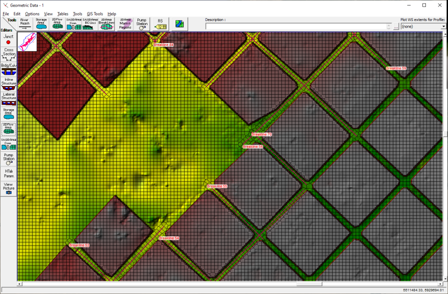
In the presence of building blocks, with no porosity, the grids are adapted to the free flood ways, as seen in this HEC-RAS example which uses breaklines as axis for the streets:

The Time Step issue

For an orthogonal or cartesian meshed domain \(\Omega\) , the Courant-Friedrichs-Levy criteria defines a CFL coefficient that linearly limits the time-step, multiplied by the cell size, and divided by the sum of flow speed and celerity:

\[ \begin{align}\begin{aligned}\Delta t_{x, y} = CFL \frac{\Delta {x, y}} {\left| U_{x, y} \right| + \sqrt{gh}}\\ \Delta t = min(\Delta t_x, \Delta t_y)_{\Omega}\end{aligned}\end{align} \]

Note that if \((\Delta {x, y}\ll, U_{x, y}\gg, h\gg )\Longrightarrow \Delta t \rightarrow 0\)

While using HEC-RAS, the time step \(\Delta t\) is controlled by a local \(CFL_i\) :

\[CFL_i=\frac{\Delta t *(\left|U_i\right|+\sqrt{gh_i}) }{\Delta x}\]

And \(\Delta t\) can be doubled or halved (with a number of fixed iterations) to satisfy for all i in the domain \(\Omega\)

\[CFL_{min} < CFL_i < CFL_{max}\]

The time-step governs the mass conservation at every control-volume or cell, for instance in 2D(X, Y):

\[\frac{\delta h} {\delta t} + \frac{\delta (hU_x)} {\delta x}+ \frac{\delta (hU_y)} {\delta y}=0\]

Whereas we go deeper with the simpler 1D(X) formulation:

\[\frac{\delta A} {\delta t} + \frac{\delta Q} {\delta x}=0\]

Which can be discretized (super-index ‘n’ stands for evolution in time and sub-index ‘i’ for location in 1D-grid) in an explicit way, like the Euler scheme :

\[\frac{ A^{n+1}_i - A^{n}_i} {\Delta t} + \frac{Q^{n}_{i+1/2}-Q^{n}_{i-1/2}} {\Delta x}=0\]

Called explicit because the value at ‘n+1’ can be formulated joining only known terms at ‘n’ on the right hand side:

\[A^{n+1}_i = A^{n}_i+ \frac{\Delta t}{\Delta x} \left( Q^{n}_{i-1/2}-Q^{n}_{i+1/2} \right)\]

Which allows for stability if \(CFL \lt 1\)

Whereas an implicit discretization scheme, like the box-scheme:

\[\begin{split}\frac{ \left( \Psi A^{n+1}_{i+1} + (1-\Psi) A^{n+1}_i \right) - \left( \Psi A^{n}_{i+1} + (1-\Psi) A^{n}_i \right)} {\Delta t} +\\ \frac{\Theta \left(Q^{n+1}_{i+1}-Q^{n+1}_{i}\right) + (1-\Theta)\left( Q^{n}_{i+1}-Q^{n}_{i}\right)} {\Delta x}=0\end{split}\]

With spatial weight \(0 \le \Psi \le 1\), and implicit parameter \(0 \le \Theta \le 1\) allows for stability even with \(CFL \gt 1\)

The price for an implicit scheme, as briefly seen, is that the solving algorithm and coding are more complex but the execution can be faster, depending also on the domain mesh division and its hardware distribution among processing units (CPU, GPU or TPU). Particularly, the popular HEC-RAS code uses an implicit scheme formulation.

Note we did not consider the conservation of momentum, for the sake of simplicity in the formulation. To know more visit[]

Simulation mass balance

One overall value to check at the end of every simulation is the mass conservation applied to the entire domain for accounting the difference of volume, and all the inflows and outflows across the boundaries.

\[V^{T} -V^{0} = \sum_k{Q^k_{in} \Delta t_k} - \sum_k{Q^k_{out} \Delta t_k}\]

Where

\[V^{n}=\sum_{\Omega}h^n_{ij}\delta x_i \delta y_j\]

Benchmarking software:

The links and credits for the referred software are:

HEC-RAS, USACE

Iber, UDC UPC CEDEX

Lisflood-FP, U. Bristol

RiverFlow2D, GHC U. Zaragoza & Hydronia Ltd

RSH-2D, US Bureau of Reclamation

TELEMAC, Global consortium